In this blog post I explain the microcontroller firmware that emulates candlelight in more detail. You can apply the explained techniques in similar situations to get organic effects on CPU and RAM-limited platforms. I will focus in my description on emulating a convincing random effects with minimal resource usage.

Table of Contents

Demo

The following video demonstrates the candlelight effect, but cameras cannot capture light situations like this very well.

Characteristics of Candlelight Flickering

If you observe a burning candle over a long time, you will notice a few key characteristics:

The flame burns in a colour range from a deep orange to a bright, almost white yellow.
The candle’s flame is usually small and orange at a low burning rate and gets higher and brighter if it increases.
Over an extended period, the burning rate varies, causing the candle to emit more or less light. Industrially produced candles have a more uniform burn rate than handmade ones.
If a draft passes the flame, it causes rapid flame flickering.
Even in closed rooms, slight air turbulence creates drafts that trigger the flame to flicker randomly.

Light that behaves in a pattern as described will trick your brain into perceiving an open burning flame.

The Hardware

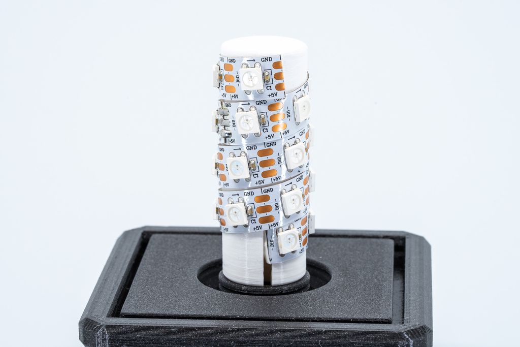
I used a strip of WS2812B RGB LED modules for the hardware that can be individually addressed.

The strip was wound around a cylinder, so the individual LEDs built five columns with four rows.

Downloads

All code examples you see on this page are from the candlelight emulator firmware you can download from GitHub:

Candlelight Emulator on GitHub

Simplification of the Overall Look

The Colour Gradient

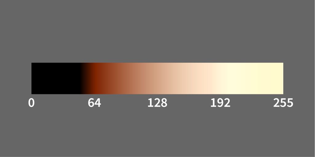
My first goal was to create a colour gradient that resembles a candle’s flame shades. The following image is a rough illustration of what I tried to archive.

For simplicity, I used a single byte as a level value and wrote a function that returns the colour for a given level.

/// Calculate the color for a given level of light intensity.
///
/// For the hue, make a transition from red to yellow.
/// For the value, go from 0 to 100%
/// for the saturation, start with 100%, then from 128, drop down to 0%.
///
/// @param level The level of the color from 0-255
/// @return The color value for this level.
///
auto colorForLevel(Level level) noexcept -> Color {
    uint16_t hue{cHueBase};
    if (level > 64) {
        hue = uint16_t{level} * cHueFactor + cHueBase;
    }
    uint8_t saturation{255};
    if (level >= uint8_t{128}) {
        saturation = uint8_t{255} - ((level - uint8_t{128}) / uint8_t{4});
    }
    uint8_t value{};
    if (level >= 192) {
        value = 255;
    } else if (level >= 64) {
        value = (level - uint8_t{64}) * uint8_t{2};
    }
    if (value < cValueCutOff) {
        return strip.Color(0, 0, 0);
    }
    return strip.ColorHSV(hue, saturation, value);
}

The function only uses multiplication and a binary-compatible division that the compiler will convert into a bit shift operation.

Create a Display with the Colours

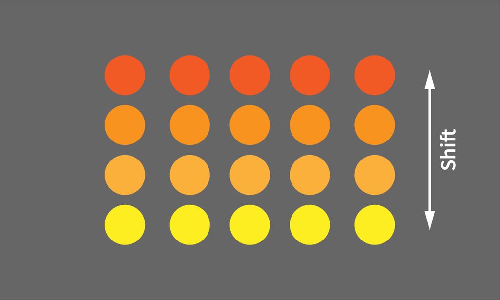
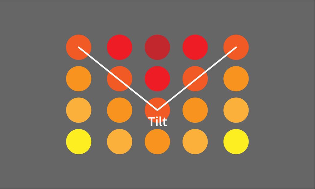
Next, I apply the colours to the individual LEDs. If I set all LEDs to the same colour uniformly, it would create a static-looking display. Therefore, I shifted the colours to make the rows look more dynamic and introduced a tilt value that added variations between the columns.

void setLevel(Level level, TiltAngle tiltAngle) noexcept {
    int16_t level16 = static_cast<int16_t>(level);
    for (int16_t row = 0; row < cLedRows; ++row) {
        int16_t rowLevel = level16 - cColorOffsetPerRow * row;
        for (int16_t column = 0; column < cLedColumns; ++column) {
            int16_t tiltFactor = static_cast<int16_t>((column <= cLedColumns / 2) ? column : (cLedColumns - column));
            int16_t tiltLevelDelta = (tiltFactor * tiltAngle) / (100 * (cLedColumns / 2));
            Level level = static_cast<Level>(clamp(rowLevel + tiltLevelDelta, 0, 255));
            auto color = colorForLevel(level);
            strip.setPixelColor(row * cLedColumns + column, color);
        }
    }
    strip.show();
}

Animate the Candle

I started working on the animation by implementing slow changes in the burning rate. Here, I created a class RandomWave that interpolates a value between changing boundaries in random durations.

Random Waves

/// A class that is generating a random wave with a defined timing and value range.
///
class RandomWave {
public:
  /// The value type created for the wave.
  ///
  using Value = int16_t;

  /// The value that the `millis()` method is using.
  ///
  using TimeValue = uint32_t;

  /// A signed time value, used for the calculation.
  ///
  /// Specified due the lack of <type_traits> in the AVR toolchain.
  ///
  using SignedTimeValue = int32_t;

  /// The configuration for the random wave.
  ///
  struct Config {
    Value minimumValue;
    Value maximumValue;
    TimeValue minimumDuration;
    TimeValue maximumDuration; 
  };

public:
  /// Create a new random wave.
  ///
  /// @param config The configuration.
  ///
  explicit RandomWave(Config config) noexcept;

public:
  /// Initialize the random wave.
  ///
  /// Call this from `setup()` once.
  ///
  /// @param currentTime The current time from the `millis()` function.
  ///
  void initialize(TimeValue currentTime) noexcept;

  /// Get the current value of the wave.
  ///
  /// Call this method from the `loop()` method.
  ///
  /// @param currentTime The current time from the `millis()` function.
  ///
  auto valueAt(TimeValue currentTime) noexcept -> Value;

private:
  /// Initialize the values for a next section of the wave.
  ///
  /// @param currentTime The current time from the `millis()` function.
  ///
  void nextRandom(TimeValue currentTime) noexcept;

private:
  Config _config; ///< The configuration.
  TimeValue _startTime; ///< The start time of the current section.
  TimeValue _currentDuration; ///< The duration for the current section.
  Value _startValue; ///< The start value for the current section.
  Value _endValue; ///< The end value for the current section.
};

The benefit of interpolating values over time is the simplicity of the implementation, making it independent of the speed of the microcontroller.

RandomWave::RandomWave(Config config) noexcept
    : _config{config}, _startTime{0}, _currentDuration{0}, _startValue{0}, _endValue{0} {
}


void RandomWave::initialize(TimeValue currentTime) noexcept {
    _startTime = currentTime;
    _endValue = static_cast<Value>(random(_config.minimumValue, _config.maximumValue));
    nextRandom(currentTime);
}


auto RandomWave::valueAt(TimeValue currentTime) noexcept -> Value {
    TimeValue timeDelta = currentTime - _startTime;
    if (timeDelta >= _currentDuration) {
        nextRandom(currentTime);
        timeDelta = 0;
    }
    SignedTimeValue factor = 1000;
    SignedTimeValue normal =
        (static_cast<SignedTimeValue>(timeDelta) * factor) / static_cast<SignedTimeValue>(_currentDuration);
    SignedTimeValue a = static_cast<SignedTimeValue>(_endValue) * normal;
    SignedTimeValue b = static_cast<SignedTimeValue>(_startValue) * (factor - normal);
    return static_cast<Value>((a + b) / factor);
}


void RandomWave::nextRandom(TimeValue currentTime) noexcept {
    _startValue = _endValue;
    _startTime = currentTime;
    _currentDuration = random(_config.minimumDuration, _config.maximumDuration);
    _endValue = static_cast<Value>(random(_config.minimumValue, _config.maximumValue));
}

The function valueAt() only requires the current time in milliseconds. Calculating a delta to the start time can interpolate the value between the start and end values with simple integer mathematics. I use a factor 1000 for the required precision of the calculations; by only using binary-compatible factors, e.g. like 256, you can further reduce the size of the generated code for some platforms.

Animate the Burning Rate

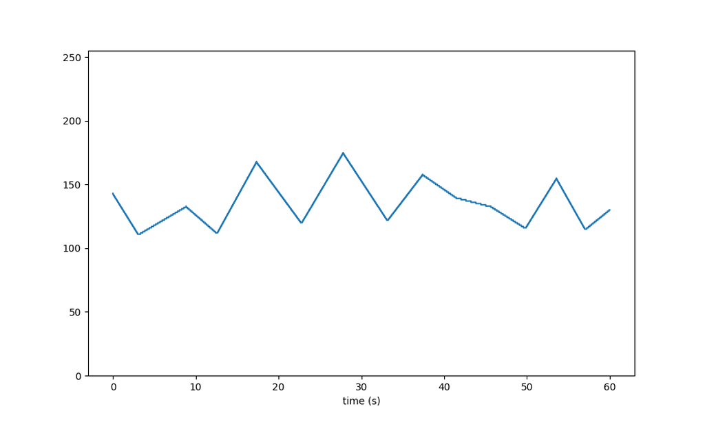
If you look at the code in the Application module, the burning rate is implemented by using an instance of the RandomWave class with the following parameters:

/// A slow random wave, emulating variations in the burn rate.
///
RandomWave gSlowWave{{100, 180, 3000, 6000}};

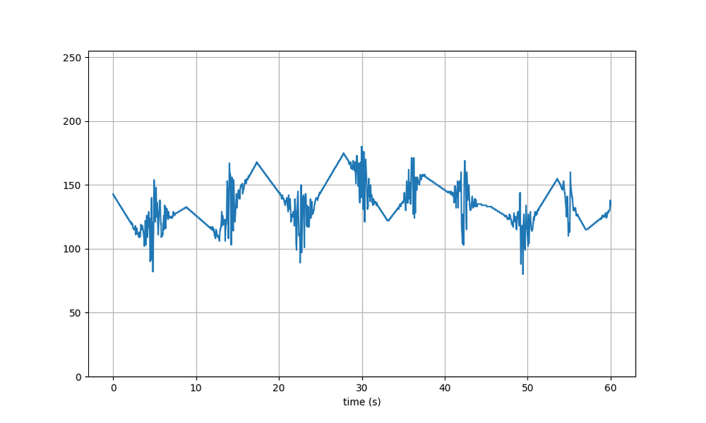
The output of this function over time looks like this:

It is a very slow shift in the brightness of the display. In the short example above, it looks as the algorithm only produces spikes, but if you look at a longer sample, you see that there are always flat shallow transitions with little change.

Animate Flickering in Draft

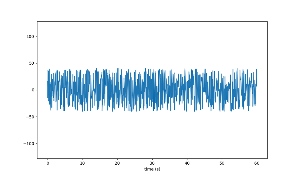
I use the same class to emulate the random flickering effect of the flame if the candle is exposed to draft.

/// A fast random wave, emulating flickering in a draft.
///
RandomWave gFastWave{{-40, 40, 20, 120}};

The shorter times with the changed start and end values will generate a fast random change in the display brightness.

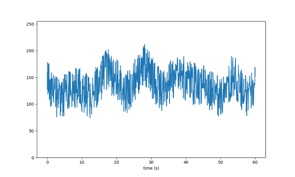
As you can see, the gFastWave instance creates a delta value, that is added to the slow changing base value of the candle.

Modulating the Draft

The result would be a candle that is permanently flickering that does not look very realistic. Therefore I added another algorithm to emulate airflow at random intervals. This class is called RandomSupressor as it suppresses the flickering most of the time.

class RandomSuppressor {
public:
    /// The value type created for the wave.
    ///
    using Value = int16_t;

    /// The value that the `millis()` method is using.
    ///
    using TimeValue = uint32_t;

    /// A signed time value, used for the calculation.
    ///
    /// Specified due the lack of <type_traits> in the AVR toolchain.
    ///
    using SignedTimeValue = int32_t;

    /// The configuration for the random wave.
    ///
    struct Config {
        TimeValue minimumDuration;
        TimeValue maximumDuration;
    };

public:
    /// Create a new random suppressor.
    ///
    /// @param config The configuration.
    ///
    explicit RandomSuppressor(Config config) noexcept;

public:
    /// Initialize the random suppressor.
    ///
    /// Call this from `setup()` once.
    ///
    /// @param currentTime The current time from the `millis()` function.
    ///
    void initialize(TimeValue currentTime) noexcept;

    /// Get the current value of the wave.
    ///
    /// Call this method from the `loop()` method.
    ///
    /// @param currentTime The current time from the `millis()` function.
    ///
    auto valueAt(TimeValue currentTime) noexcept -> Value;

private:
    /// Initialize the values for a next section.
    ///
    /// @param currentTime The current time from the `millis()` function.
    ///
    void nextRandom(TimeValue currentTime) noexcept;

private:
    Config _config; ///< The configuration.
    TimeValue _startTime; ///< The start time of the current section.
    TimeValue _currentDuration; ///< The duration for the current section.
};

The implementation of this class is very similar to RandomWave:

RandomSuppressor::RandomSuppressor(RandomSuppressor::Config config) noexcept
    : _config{config}, _startTime{0}, _currentDuration{0} {
}


void RandomSuppressor::initialize(RandomSuppressor::TimeValue currentTime) noexcept {
    _startTime = currentTime;
    nextRandom(currentTime);
}


auto RandomSuppressor::valueAt(RandomSuppressor::TimeValue currentTime) noexcept -> RandomSuppressor::Value {
    TimeValue timeDelta = currentTime - _startTime;
    if (timeDelta >= _currentDuration) {
        nextRandom(currentTime);
        timeDelta = 0;
    }
    constexpr Value factor = 1000;
    SignedTimeValue normal =
        (static_cast<SignedTimeValue>(timeDelta) * factor) / static_cast<SignedTimeValue>(_currentDuration);
    if (normal >= (factor / 2)) {
        normal = factor - normal;
    }
    normal *= 2;
    normal = (normal * normal) / factor; // quad1
    normal = (normal * normal) / factor; // quad2
    return static_cast<Value>(normal);
}


void RandomSuppressor::nextRandom(RandomSuppressor::TimeValue currentTime) noexcept {
    _startTime = currentTime;
    _currentDuration = random(_config.minimumDuration, _config.maximumDuration);
}

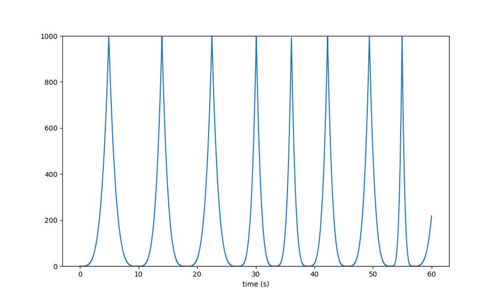
I work with a fixed value range from zero to 1000 that act as a normalization value used to modulate the flickering. An initial symmetric triangle waveform is interpolated between random time intervals. By calculating the cubic result two times, the triangle is transformed in a series of spikes.

/// A peak suppressor, emulating random drafts passing the candle.
///
RandomSuppressor gSuppressor{{3000, 10000}};

The result of gSuppressor looks like this:

Combining all Results

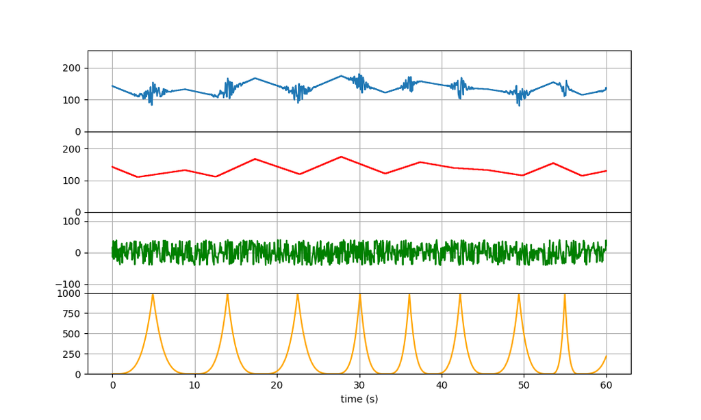
When all results are combined, the brightness value for the display looks like this:

I combined all generated values in one diagram so you can see its individual influences on the result.

Now shown is the fourth waveform for the tilt effect. This last one is very subtle and slow moving, adding more variation to the light.

Conclusion

The four individual random interpolated waveforms are simple to implement and the resulting code fits into the 5kb flash memory of the Adafruit Trinket I used for me experiments. With each additional generator, the results gets more organic and looks more natural.

Working with minimalistic generator code like this is not only useful for small microcontrollers, but also an interesting way to write integer based filter effects. If you have questions, missed any information, or wish to provide feedback, add a comment below or send me a message.