published: December 30, 2021 —
last modified: October 23, 2025
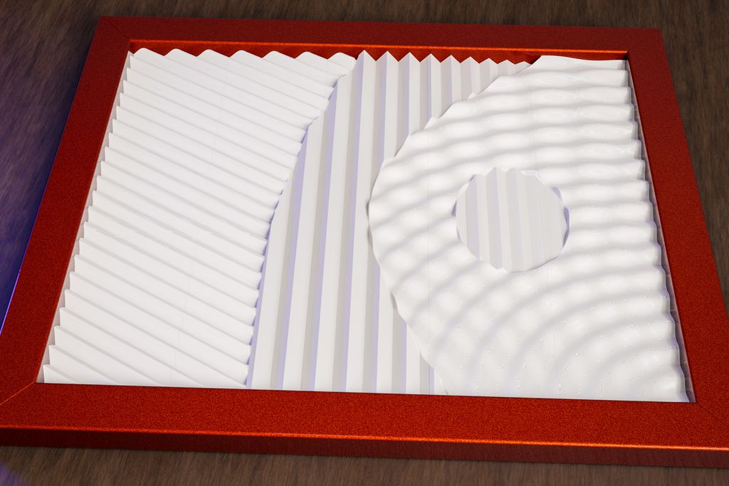
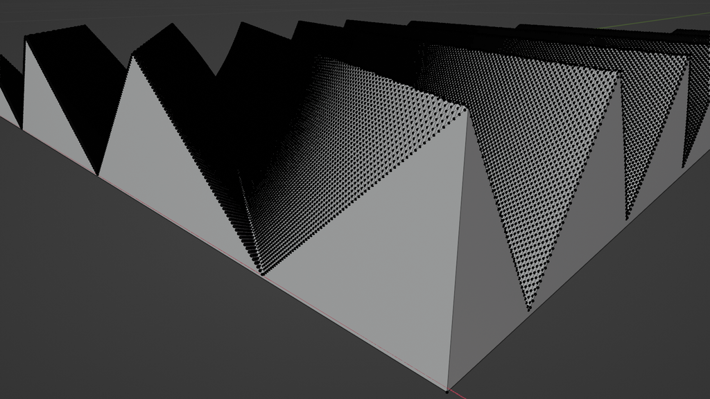
I recently built a relatively large (100cm × 80cm) 3D printed artwork, which features a painted relief of mathematical functions. Read how I prepared the data, converted it into 3D printable tiles and converted them into printable gcode.
All the images and previews are from the proof of concept I created. The final artwork is quite different, but I used the same code and methods to develop it.
In this short tutorial, I will focus on the technical aspects to create the 3d printed tiles, including the scripts I used. I will only briefly cover the assembly and painting process, as I think this is too much out of the scope of my blog.
Table of Contents
My Vision
Since working with computers, I have always liked two or three dimensions function plots of mathematical formulas. When I got a 3D printer, I tried various ways to create something physical from mathematical data. After creating smaller art pieces, I had to test something larger.
My idea was to visualize three different functions on a larger canvas. The abstract artwork has three distinct sections, and each of these sections has its colour and mathematical formula.
Define the Picture Dimension
As all the calculations and generation of the data and models will be complex, I first set the final dimensions of the artwork. I found 100cm × 80cm is a good size, large enough to impress, but still light enough to hang on a wall.
Next, I tested various data resolutions and how they look printed: A one-millimetre data resolution was just a little bit too large to create a smooth surface, so I set it to 0.5mm. Yet, I also found that larger data resolutions of 10mm create a unique effect, and it is something I will try at a later time.
Prepare the Function Data
I started creating the functions. Here, I used a simple python script to create a two-dimensional preview image of the function.
importnumpyasnpimportimageioasiiofrommathimportsin,pi,sqrt,radiansfrompathlibimportPath# SettingsDATA_WIDTH=2000# pointsDATA_HEIGHT=1600# pointsPROJECT_DIR=Path(__file__).parentPREVIEW_IMG_PATH=PROJECT_DIR/'function_preview.png'classWorkingSet:def__init__(self):self.out_img=np.zeros(shape=(DATA_HEIGHT,DATA_WIDTH,3),dtype=np.uint8)@staticmethoddefget_z(x:float,y:float)->float:"""
Function to generate the z height.
@param x The input in the range 0.0-1.0
@param y The input in the range 0.0-1.0
@return The result in the range 0.0-1.0.
"""d=sqrt((1-x)**2+y**2)d1=sqrt((1-x)**2+y**2)d2=sqrt((1-x-0.6)**2+(y+0.1)**2)f1=sin(radians(d1*16*360))f2=sin(radians(d2*17*360))f=(((f1+f2*0.3)/2.0)+1.0)/2.0z=f*((d/sqrt(2)*0.78)+0.5)returnzdefrun(self):"""
Run this working set.
"""print('Calculate function data...')out=np.zeros(shape=(DATA_HEIGHT,DATA_WIDTH))forpyinrange(DATA_HEIGHT):forpxinrange(DATA_WIDTH):z=self.get_z(px/(DATA_WIDTH-1),1.0-py/(DATA_HEIGHT-1))ifz>1.0:z=1.0ifz<0.0:z=0.0out[py,px]=zprint('Create visualization...')foryinrange(DATA_HEIGHT):forxinrange(DATA_WIDTH):z=out[y,x]self.out_img[y,x]=[np.uint8(z*255),np.uint8(z*255),np.uint8(z*255)]iio.imwrite(str(PREVIEW_IMG_PATH),self.out_img)defmain():working_set=WorkingSet()working_set.run()if__name__=='__main__':main()
The script has a simple “settings” section, where I define the primary parameters of the preview. The shown case is 2000 by 1600 pixels, which match the 0.5mm resolution for the 100cm × 80cm picture.
In get_z I define the function to create the Z-value for each image pixel. It takes normalized values from 0.0 to 1.0 and returns values in the range of 0.0 to 1.0.
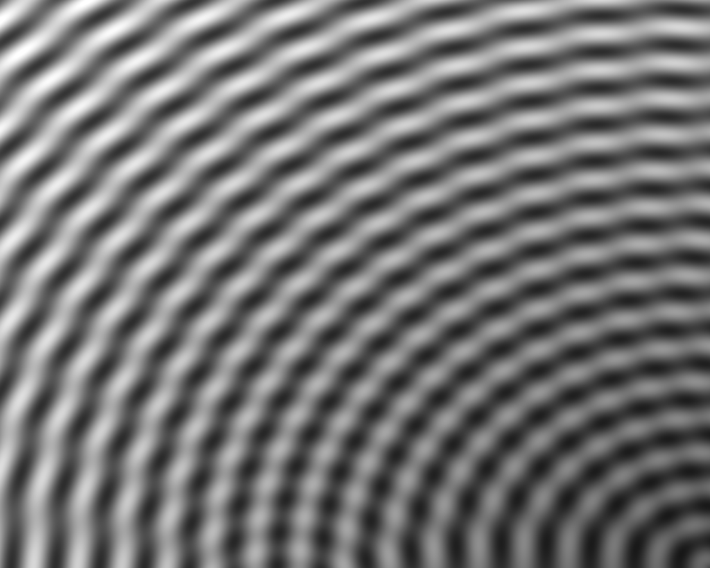
The preview script generates this image.
I used this simple preview script to create all three formulas. Yet, the visualization is not perfect because a grayscale image does not correctly visualize height levels.
Prepare the Sections
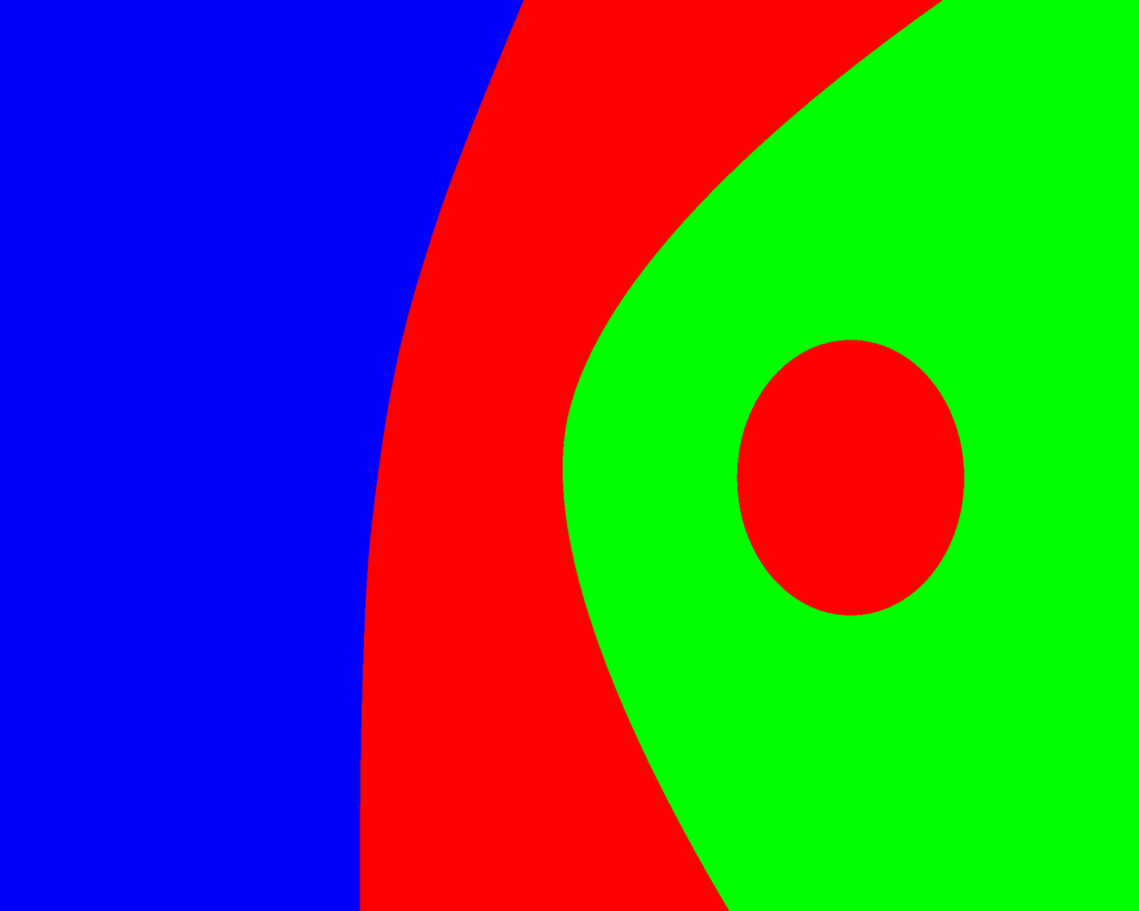
To visualize the colours and sections of the final image, I created a simplified representation in a vector drawing program. Then, I made an even simpler version for the calculations, only consisting of red, blue, and green areas. Next, I exported it as a PNG image with 2000 × 1600 pixels without antialiasing.
The image above defines the function sections.
Calculate the Picture Relief
Next, I calculated the Z-data for the whole picture, combining all three functions into one. I used the following python script for this calculation:
importenumfromtypingimportOptionalimportnumpyasnpimportimageioasiiofrommathimportsin,pi,sqrt,radiansfrompathlibimportPath# SettingsPICTURE_WIDTH=1.0# mPICTURE_HEIGHT=0.8# mRELIEF_HEIGHT=0.03# mRELIEF_BASE_THICKNESS=0.002# mPICTURE_RESOLUTION=0.0005# mDATA_WIDTH=2000# pointsDATA_HEIGHT=1600# pointsPROJECT_DIR=Path(__file__).parentSECTION_WIDTH=DATA_WIDTH# pxSECTION_HEIGHT=DATA_HEIGHT# pxSECTION_PATH=PROJECT_DIR/'sections.png'PREVIEW_IMG_PATH=PROJECT_DIR/'preview_image.png'Z_DATA_PATH=PROJECT_DIR/'z_data.npy'SECTION_BLEND_PATH=PROJECT_DIR/'section_blend_data.npy'SECTION_BLEND_SIZE=3# delta pixelsclassSection(enum.Enum):NONE=0RED=1GREEN=2BLUE=3classWorkingSet:def__init__(self):self.img:Optional[np.ndarray]=Noneself.blend:Optional[np.ndarray]=Noneself.out_img=np.zeros(shape=(DATA_HEIGHT,DATA_WIDTH,3),dtype=np.uint8)@staticmethoddefget_blue_z(x:float,y:float)->float:"""
Function to generate the z height for the blue section.
@param x The input in the range 0.0-1.0
@param y The input in the range 0.0-1.0
@return The result in the range 0.0-1.0.
"""defwave(v:float):n=(v+0.5)%1.0return(nifn<0.5else1.0-n)*2.0d=(x+y*1.46)*15f1=(sin(radians(d*360))+1.0)/2.0f2=wave(d)z=((f1*y)+(f2*(1.0-y)))*((1.0-y)*0.3+0.7)returnz@staticmethoddefget_red_z(x:float,y:float)->float:"""
Function to generate the z height for the red section.
@param x The input in the range 0.0-1.0
@param y The input in the range 0.0-1.0
@return The result in the range 0.0-1.0.
"""defwave(v:float):n=v%1.0return(nifn<0.5else1.0-n)*2.0h=abs(sin(radians(x*1.2*180)))*0.8+0.2d=sin(radians((x+0.1)*360))*0.7returnwave(x*25+d)*h@staticmethoddefget_green_z(x:float,y:float):"""
Function to generate the z height for the green section.
@param x The input in the range 0.0-1.0
@param y The input in the range 0.0-1.0
@return The result in the range 0.0-1.0.
"""d=sqrt((1-x)**2+y**2)d1=sqrt((1-x)**2+y**2)d2=sqrt((1-x-0.6)**2+(y+0.1)**2)f1=sin(radians(d1*16*360))f2=sin(radians(d2*17*360))f=(((f1+f2*0.3)/2.0)+1.0)/2.0z=f*((d/sqrt(2)*0.8)+0.5)returnzdefget_section(self,px:int,py:int)->Section:"""
Get the section based on a pixel in the section image.
:param px: The pixel in the x axis (0-image width)
:param py: The pixel in the y axis (0-image height)
:return: 0 for no section (out of bounds), 1, 2, 3 for a coloured section.
"""ifpx<0orpx>=SECTION_WIDTHorpy<0orpy>=SECTION_HEIGHT:returnSection.NONEp=self.img[py,px]ifp[0]>=128:returnSection.REDifp[1]>=128:returnSection.GREENreturnSection.BLUEdefcalculated_blended_row(self,py:int)->np.ndarray:"""
Calculate a row from the section file, blending the surrounding pixels into
a function weighting map.
:param py: The pixel row in the y axis.
:return: An array with function weights for all three functions.
"""row=np.zeros(shape=(DATA_WIDTH,3))forpxinrange(DATA_WIDTH):found_pixels=0foryinrange(py-SECTION_BLEND_SIZE,py+SECTION_BLEND_SIZE+1):forxinrange(px-SECTION_BLEND_SIZE,px+SECTION_BLEND_SIZE+1):m=self.get_section(x,y)ifm==Section.NONE:continuefound_pixels+=1row[px,m.value-1]+=1iffound_pixels>0:row[px]/=found_pixelsreturnrowdefget_z(self,px:int,py:int)->float:"""
Calculate the z height for a given pixel.
:param px: The x coordinate for the pixel.
:param py: The y coordinate for the pixel.
:return: The z value for the given pixel coordinates.
"""m=self.blend[py,px]x=px/(DATA_WIDTH-1)y=1.0-(py/(DATA_HEIGHT-1))z=(self.get_red_z(x,y)*m[0])+(self.get_green_z(x,y)*m[1])+(self.get_blue_z(x,y)*m[2])z/=(m[0]+m[1]+m[2])ifz<0:z=0ifz>1.0:z=1.0returnzdefrun(self):"""
Run this working set.
"""ifSECTION_BLEND_PATH.is_file():print('Reading blend data...')self.blend=np.load(str(SECTION_BLEND_PATH))else:print('Generating blend data...')self.img=iio.imread(SECTION_PATH)self.blend=np.ndarray(shape=(DATA_HEIGHT,DATA_WIDTH,3))forpyinrange(DATA_HEIGHT):print(f'at row {py}...')self.blend[py]=self.calculated_blended_row(py)np.save(str(SECTION_BLEND_PATH),self.blend)print('Calculate functions...')out=np.zeros(shape=(DATA_HEIGHT,DATA_WIDTH))forpyinrange(DATA_HEIGHT):forpxinrange(DATA_WIDTH):out[py,px]=self.get_z(px,py)np.save(str(Z_DATA_PATH),out)print('Create visualization')foryinrange(DATA_HEIGHT):forxinrange(DATA_WIDTH):z=out[y,x]self.out_img[y,x]=[np.uint8(z*255),np.uint8(z*255),np.uint8(z*255)]iio.imwrite(str(PREVIEW_IMG_PATH),self.out_img)defmain():working_set=WorkingSet()working_set.run()if__name__=='__main__':main()
I use three functions get_blue_z, get_red_z and get_green_z to for the different z-profiles of the three sections.
After the start, I read the section data from the image sections.png, adding a small “blur effect” and converting them into a weight map. This map contains three values for each data point. Each value controls the amount used from each function. Converting these values can take quite a while. Therefore I store them in the file section_blend_data.npy for later use.
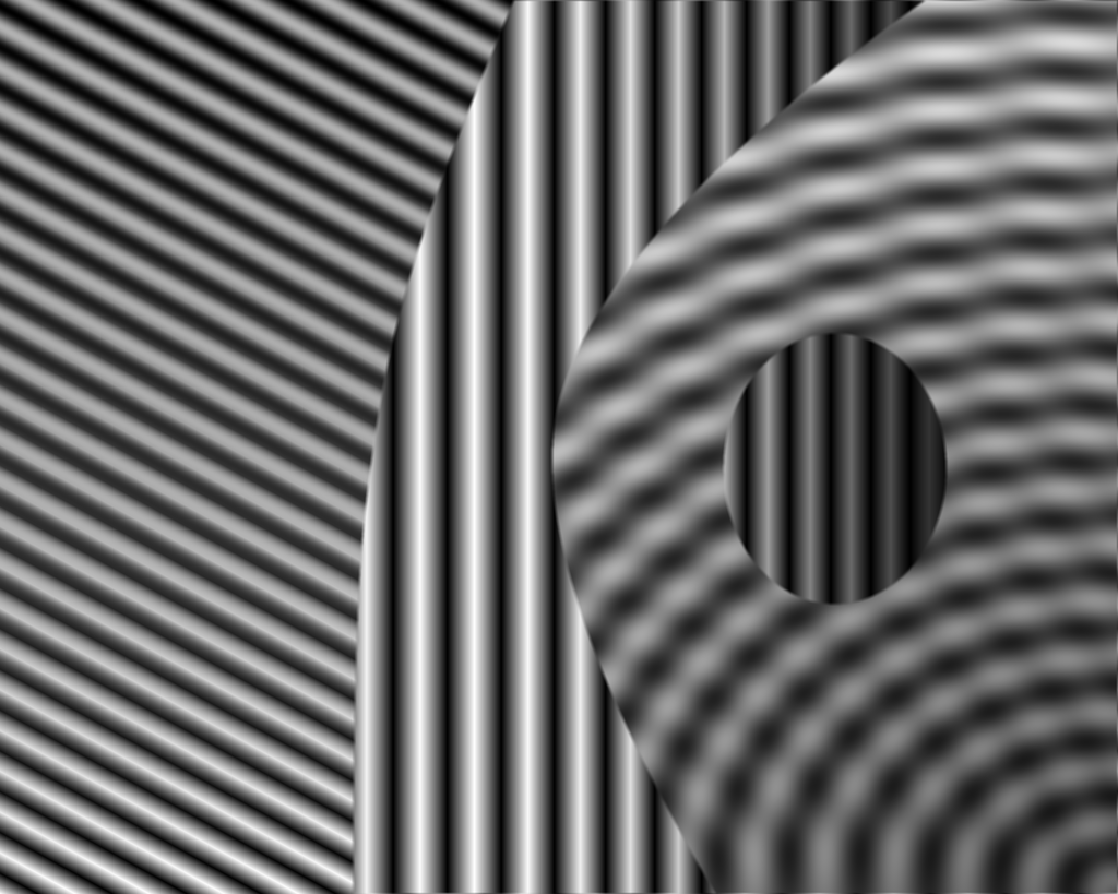
Next, I use the weight map to calculate the final z-values for all data points. From these values, I create another preview image preview_image.png and also store them in the file z_data.npy.
The preview image looks like this:
The final preview image.
Convert the Data into 3D Objects
Next, I switched to Blender to create 3D objects from the data. Here I used a simple script, creating individual tiles from the data:
importbpyimportnumpyasnp# SettingsRELIEF_HEIGHT=0.03# mRESOLUTION=0.0005# mBASE_THICKNESS=0.0006# mTILE_SPACING=0.0002# mZ_DATA=np.load('<path>/z_data.npy')Z_DATA_WIDTH=2000# pxZ_DATA_HEIGHT=1600# pxdefget_z(x:float,y:float)->float:"""
Get the Z value for a data point.
:param x: The x coordinate in data space.
:param y: The y coordinate in data space.
:return: The resulting Z value in model space.
"""ifx<0:x=0ify<0:y=0ifx>=(Z_DATA_WIDTH-1):x=Z_DATA_WIDTH-1ify>=(Z_DATA_HEIGHT-1):y=Z_DATA_HEIGHT-1z=float(Z_DATA[Z_DATA_HEIGHT-y-1,x])*RELIEF_HEIGHTreturnzdefcreate_tile(sx:int,sy:int,width:int,height:int,name:str):"""
Create a tile with start sx, sy and width, height in shape units
"""vert_width=width+1vert_height=height+1defget_vert_index(x:int,y:int)->int:"""
Get the vertice index for one coordinate.
"""returnx*vert_width+ydefface(x:int,y:int):"""
Get one face tuple on the surface.
"""return(get_vert_index(x,y),get_vert_index(x+1,y),get_vert_index(x+1,y+1),get_vert_index(x,y+1))defget_point(x:int,y:int):"""
Get one single point in model space.
"""rx=(sx+x)*RESOLUTIONifx==width:rx-=TILE_SPACINGry=(sy+y)*RESOLUTIONify==height:ry-=TILE_SPACINGrz=get_z(sx+x,sy+y)returnrx,ry,rz# Create the vertices for the surface.vertices=[get_point(x,y)forxinrange(vert_width)foryinrange(vert_height)]faces=[face(x,y)forxinrange(width)foryinrange(height)]# Add four vertices for the bottombt_index=len(vertices)# Store the index of these four bottom vertices.x1=sx*RESOLUTIONx2=(sx+width)*RESOLUTION-TILE_SPACINGy1=sy*RESOLUTIONy2=(sy+height)*RESOLUTION-TILE_SPACINGvertices.extend([(x1,y1,-BASE_THICKNESS),(x2,y1,-BASE_THICKNESS),(x2,y2,-BASE_THICKNESS),(x1,y2,-BASE_THICKNESS)])# add all other sides# fronttop_edge=[get_vert_index(vert_width-x-1,0)forxinrange(vert_width)]top_edge.extend([bt_index,bt_index+1])faces.append(top_edge)# backtop_edge=[get_vert_index(x,vert_height-1)forxinrange(vert_width)]top_edge.extend([bt_index+2,bt_index+3])faces.append(top_edge)# lefttop_edge=[get_vert_index(0,y)foryinrange(vert_height)]top_edge.extend([bt_index+3,bt_index])faces.append(top_edge)# righttop_edge=[get_vert_index(vert_width-1,vert_height-y-1)foryinrange(vert_height)]top_edge.extend([bt_index+1,bt_index+2])faces.append(top_edge)# bottomfaces.append([bt_index,bt_index+3,bt_index+2,bt_index+1])# Create Mesh Datablockmesh=bpy.data.meshes.new(name)mesh.from_pydata(vertices,[],faces)# Create Object and link to sceneobj=bpy.data.objects.new(name,mesh)bpy.context.scene.collection.objects.link(obj)defmain():tile_width=400tile_height=400forxinrange(5):foryinrange(4):create_tile(tile_width*x,tile_height*y,tile_width,tile_height,f'tile{y}{x}')if__name__=='__main__':main()
What didn’t Work
Originally I started with a different approach, where I created one solid object with the profile. Then, I made boxes in the correct sizes of the tiles and boolean operations to convert the relief into smaller entities.
While this approach seemed more straightforward and accurate, Blender could not produce correct geometrical results. The created tiles always had defects, which caused problems in the slicer. Repairing these defects was time-consuming, but I also had to fix the objects after every rebuild of the geometries manually.
My Blender script is as simple as possible. It loads the generated Z-data into a NumPy array, creating separate tiles.
Instead of working with actual dimensions and dividing them into the data points, I define the distance between the data points using the variable RESOLUTION.
I create each tile by generating a grid of vertices, using the Z-values multiplied with the desired relief size. Next, I add faces between all the vertices to build the top surface of the tile.
Now I add four vertices more at the four bottom corners of the object. Then I create faces on the sides, connecting all the vertices from the side of the top surface with two vertices at the bottom.
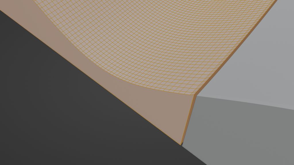
I move the vertices on the top and right sides by a tiny amount to create a minimal gap between the tiles. This gap is required to compensate for printing variations and the glue.
Reduce the Mesh Size?
I found reducing the mesh size is not worth the time and effort. The slicer software can efficiently deal with complex objects like these. Also, because the grid never perfectly represents the functions, I found changing the faces will often make these imperfections more visible.
Export the Tiles from Blender
Exporting all the tiles from Blender is simple. The export dialogue has a batch function, where you can save a selection of objects into individual files.
So, I export all the generated tiles in individual STL files. I name them picture_tileXX.stl. In the Blender export dialogue, I use picture_.stl as filename, where it automatically adds the name of the objects at the end of this name.
Slicing the Tiles
Next, I slice all the objects and convert them into gcode. I first import one of the STL files in Prusa Slicer and configure all required parameters. After I am happy with the slicing results, I store the configuration with “File”->“Export”->“Export Config…” into a config.ini file.
Now I can use the following Python script to convert all files into gcode automatically:
Printing all the 20 tiles took some time, but watching how the relief emerges layer by layer is lovely.
After each print, I wrote the tile number on its back, which was a great help with the assembly.
Assemble and Paint the Tiles
I used a slightly larger sheet of plywood to assemble the tiles into the painting. I put all the tiles into place, using a fast curing epoxy glue.
Next, I smoothed the surface with sandpaper. Smoothing the surface also removed most of the small tips from the seams. Where required, I filled the small gap between the tiles with wood filler. Adding a primer further smoothed the surface.
I used acrylic colours to paint the relief with the colours I wanted. These colours nicely separated the different reliefs and added more depth and detail.
Conclusion
I hope this short tutorial gave you the inspiration to create your own large 3d painting. The final result at this scale is very impressive and with the large structures, the painting looks very different depending on the lights and its shadows.
If you have any questions, missed information, or simply want to provide feedback, feel free to comment below. 😄
I built a small compiled command-line tool to read SHT31 temperature and humidity over I2C on a Raspberry Pi. It emits simple JSON for easy parsing in scripts. If you're using an SHT31 sensor or automating reads, read the full post for usage, build and install steps.
Posted on 2019-07-12— C++, Improve your Code, Learn
I walk through practical ways I use C++11's auto keyword to reduce repetitive declarations, simplify range-based for loops, lambdas and register access, and make Arduino and embedded code easier to refactor. Read the full post for examples and tips you can apply to your projects.
Posted on 2019-07-08— C++, Improve your Code, Learn
I guide you through evolving a simple Arduino blink example into a reusable event system. In Part 2 I cover function-pointer events, an EventLoop module, and practical multi-event examples. If you want cleaner, non-blocking firmware structure, read the full post for code and explanations.
Posted on 2019-07-29— C++, Improve your Code, Learn
I explain C++11 enum class: why it prevents name conflicts, how it compares to traditional enums and common workarounds, with practical Arduino-friendly examples. If you want clearer, safer enum usage in your interfaces, read the full post for code samples and simple best-practice guidance.
I've created a collection of 3D-printable flower pots—geometric, Roman-vase inspired, striped and spiral—optimized for practical printing on machines like the Prusa XL. I share lessons on wall thickness, corner radii, nozzle sizes and model files. Read on for design details and downloads.
Posted on 2023-01-29— 3D Printing, Build, Projects
I tested three inexpensive, easy methods to add LED lighting to my modular 3D‑printed lantern using USB power: reused LED modules, short 5V strips, and WS2812B RGB with a microcontroller. I share parts lists, soldering tips, diffuser advice, and firmware steps—read on for step‑by‑step instructions and printable models.